Automatic Serial Numbers in Excel

Last Updated on 3 years by admin

If you are maintaining a list of customers or constantly changing list of items, this Excel Trick is for you. Automated Serial Numbers in MS Excel will save you from the pain that you are used to go through each time when there’s a new ROW is added or removed.

Let’s check out how easy this Trick is.

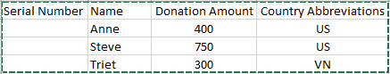
1. Open excel and add the columns that you need and fill out few rows. In the example that is listed below shows Donation list that frequently changes

2. Once the Columns are created and the rows are updated select the area and press Ctrl + T (Control button & the Character button T) and press ‘OK. This will create the table.
   
3. On the 1st Row of the Column that you need to add serial numbers. Type the following command =ROW()-ROW(Slecect the header column ‘serial number’ and close the bracket) then press enter. It will create the serial number list. It should look similar to =ROW()-ROW(Table5[[#Headers],[Serial Number]])
4. Now the list of serials should display. Now try adding more rows or deleting rows and the ‘Serial Numbers’ should auto populate. Also, the ‘Serial Number’ column is moveable without an issue.

Jump to next Excel Trick